Elements of Electromagnetism (II)

by Mel

I would like to continue the discussion I started here about electromagnetism. Last time I stoped right when things were getting interesting: we had reached special relativity. Some words about special relativity follow.

Einstein realized that electromagnetic disturbances propagated with the same (constant) speed always (in vacuum) and that if one had two observers whose frames of reference were inertial with respect to each other their time and spatial coordinates were not rigid and had to fuse together into what was later called spacetime. Longest. Sentence. Ever. The fusion of space and time into spacetime then requires the introduction of an indefinite, Lorentzian metric instead of the cherished Euclidean metric. Spacetime intervals are invariant under a “bigger” symmetry called Lorentz symmetry which includes “rotations” between the spatial and the temporal dimensions. In some way, this business reduces to writing temporal and spatial “stuff” with just one symbol, in a way that the Lorentz symmetry is exhibited. For example we now use:

$x^\mu = \left(t, \vec{x}\right)$ and $\partial_{\mu} = \left(\displaystyle\frac{\partial }{\partial t}, \nabla\right)$ .

As we can see the trend is to combine a 3-vector with a scalar quantity. For electromagnetism we have many important 3-vectors. It turns out that the electric and the magnetic fields do not compose a “four-vector”. Instead we can introduce the four-potential and the four-source:

$A^{\mu} = \left(\phi, \vec{A}\right)$ and $J^{\mu} = \left(\rho, \vec{J}\right).$

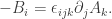
With these we can use the four-derivative to write expressions for the electric and magnetic fields. Because of the indefinite metric we have $A_{0} = - A^{0}$ . Then using these symbols we have

$- E_{i} = \partial_{0} A_{i} - \partial_{i} A_{0}$ and $-B_{i} = \epsilon_{ijk}\partial_{j}A_{k}.$

These two expressions can be shown to be different components of the same thing: the electromagnetic field strength, AKA the Faraday tensor. This tensor is defined by

$F_{\mu\nu} = \partial_{\mu}A_{\nu} - \partial_{\nu}A_{\mu}.$

Some might call it notation, but in this covariant form it is very clear that the electric and the magnetic fields are just aspects of the same thing: the field strength. In my humble opinion, true “unification” was achieved the moment one pairs the scalar and vector potentials into the four-potential and similarly for the four-source.

How do Maxwell’s equations look like in terms of the field strength? The answer is quite beautiful:

$\partial_{\mu} F^{\mu \nu} = J^{\nu}$ and $\partial_{[\mu}F_{\sigma \rho ]} = 0,$

with the square brackets in the second expression mean antisymmetrization in the indices. Sometimes people introduce the dual field strength,

$G_{\mu \nu} = \displaystyle\frac{1}{4!} \epsilon_{\mu\nu\sigma\rho}F^{\sigma\rho},$

but this notation is not that helpful. Maybe in terms of differential forms it means something, but I will leave that for later.

Gauge invariance now means that both

$A_{\mu}$ and $A_{\mu}' = A_{\mu} + \partial_{\mu}\lambda$

give the same field strength. Indeed, this is true as long as partial derivatives commute and hence Maxwell’s equation are invariant under a gauge transformation. Honestly, besides thinking of the electric and the magnetic fields as different aspects of the same thing, we have found nothing new. In a way Special Relativity is just basically writing down all the previously known stuff in a better notation (and treating space and time equally).

We have talked to many undergraduates and they have told us about electromagnetism and its different manifestations. (You have to read the previous post on this topic to get this comment.) You might be thinking something along the following: “electromagnetism is elegant but honestly, kind of boring…”. That is actually true. The electric and the magnetic field affect each other, but besides one serving as the “source” of the other, there is not that much else to study. So now you wonder what the graduate students learn in their quantum mechanics class. After asking one of these so-called “grad-students” one reacts with puzzlement with their reply: “The quantum realm is where electromagnetism gets really interesting!”.

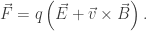
How do the electric and magnetic fields interact with a charge particle? Well, the dynamics of such a charged particle in the presence of external electric and magnetic fields (I.E. the particle does not interact with the field it produces) is governed by the Lorentz force:

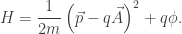
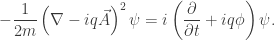
$\vec{F} = q\left(\vec{E} + \vec{v} \times \vec{B}\right).$

There is a Hamiltonian function that gives this equation of motion:

$H = \displaystyle\frac{1}{2m}\left(\vec{p} - q \vec{A}\right)^2 + q \phi.$

This is certainly interesting in the classical realm, but when we promote this Hamiltonian to a quantum-mechanical operator we get something that is truly beautiful. Recall the Schrödinger equation:

$\hat{H}\psi = i\displaystyle\frac{\partial \psi}{\partial t}.$

If you know a bit of physics you might object now: why use the Schrödinger equation after going through the ordeal of writting everything in a nice covariant way? The Schrödinger equation is non-relativistic. But what I am going to do with it can be done with any equation you like (I hope…); this works with the Dirac equation and with the Klein-Gordon equation. (Actually, this only works for what physicist like to call “spin-0” and “spin-1/2” cases.)

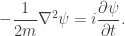
One can go from a classical Hamiltonian to the Schrödinger equation by using $\vec{p} \rightarrow -i \nabla$ and usually one does not get in trouble. In our case we are going to assume that the vector potential is a smooth function of the coordinates and not of the derivatives of the coordinates. We will also put any ordering ambiguities in our back pockets and sit on them while we read this post. Then, for a charged particle, the Schrödinger equation reads (in a very suggestive form)

$-\displaystyle\frac{1}{2m}\left( \nabla - i q \vec{A}\right)^2 \psi = i \left(\displaystyle\frac{\partial}{\partial t} + iq\phi\right) \psi.$

The expression above can be compared to the free-particle case:

$-\displaystyle\frac{1}{2m}\nabla^2 \psi = i \displaystyle\frac{\partial \psi}{\partial t}.$

We see that naively we can go from the free particle Schrödinger to the charged-particle case by changing

$\nabla \Rightarrow \nabla - i q \vec{A}$ and $\displaystyle\frac{\partial}{\partial t} \Rightarrow \displaystyle\frac{\partial}{\partial t} + iq\phi.$

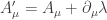
This will turn out to be a very helpful “rule-of-thumb” later. Now, what about the gauge invariance exhibited by Maxwell’s equations, will it carry over to the quantum realm? If we consider two sets of potentials, $(\phi, \vec{A})$ and $(\phi', \vec{A}')$ , related by a gauge transformations:

$\vec{A}' = \vec{A} + \nabla \lambda$ and $\phi' = \phi - \displaystyle\frac{\partial \lambda}{\partial t},$

then we can see that for the Schrödinger equation to have the same form for both set of potentials we also need to required

$\psi' = \exp{\left( i q \lambda\right)} \psi.$

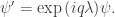
This expression relates the wavefunctions of each gauge choice. You look at this for a while. What does it mean? One way to look at it is as follows: under a gauge transformation, the wavefunction gets a phase factor that depends on the position of space and time.

Is the physics changing under this gauge transformation? The answer is a surprising no. Recall that the physical content of the wavefunction comes not from the wavefunction itself, but from the square of its modulus. A phase washes off this modulus. So together with this “local” phase, both systems describe the same physics.

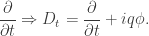
One may argue that if you consider an operator that contains space and time derivatives then this local phase will definetely play some role and then expectation values in both systems will not agree. To “fix” this one uses the following rule: change all derivative operators to “gauge-covariant derivative” operators:

$\nabla \Rightarrow \vec{D} = \nabla - i q \vec{A}$ and $\displaystyle\frac{\partial}{\partial t} \Rightarrow D_{t} = \displaystyle\frac{\partial}{\partial t} + iq\phi.$

This way the contribution of the phase cancels out and the expectation values of operators will agree in both systems. So we have found that gauge invariance of Maxwell’s equations holds in the quantum realm as long as we allow the wavefunction to change by a local phase factor the precisely depends on the gauge parameter. These rules make the Schrödinger equation gauge invariant. A very similar process can be done for the Dirac equation. Homework perphaps?

What if we now reverse the argument? That is, start from the free particle Schrödinger and impose the following “physical law”:

The physical content of the Schrödinger equation is invariant under a phase transformation.

First of all, what type of phase transformation? Local or global? For a global phase (a constant) it is straightforward to show that this change does not affect anything. The phase drops off from the modulus also. Meanwhile, for a local phase the Schrödinger equations are going to look different in both systems since the derivatives operate on the spatially- and time-dependent phase. By introducing this local phase we are effectively changing the phase of the wavefunction at each point in space and across time also. This sounds like…

…not a free particle at all! Then our particle is interacting with something, some set of fields. We already know what are these fields: the scalar and vector potentials. These are the fields that are needed to make the physics invariant under this local phase transformation. So by impossing a local symmetry we have arrived at an interacting theory: electromagnetic interactions of a charged, Schrödinger particle are the concequence of local phase invariance of the wavefunction! Some nomenclature: since the scalar and vector potentials can be “gauged” by a gauge transformation, we call this set of fields gauge fields.

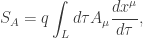
It is in this sense that electromagnetism can be viewed as a gauge theory with gauge field $A_{\mu}$ . When electromagnetism is coupled to scalar or spinor fields, it corresponds to the gauge theory of local phase invariance. Indeed, the strong and weak interactions are currently best understood as gauge theories of local “non-abelian phases”. The significance of this term will be explain later. For now one needs to know that Maxwell theory is also knows a abelian gauge theory.

Let us start our decend from the clouds by going back to the Schrödinger equation for a charged particle. Imagine that our vector potenial is given by the gradient of some scalar function. By definition, the magnetic field will vanish:

$\vec{A} = \nabla f \Rightarrow \vec{B} = 0.$

We can write the solution to the Schrödinger equation in terms of the free-particle wavefunction $\psi_{0}$ :

$\psi = \exp{\left(i q \displaystyle\int_{-\infty}^{x}\nabla f \cdot d\vec{y}\right)}\psi_{0}.$

Recall that

$\nabla f \cdot d\vec{y} = df.$

Then the integral can be done. The end result of this particular vector potential is to multiply the free-particle solution by a phase that is local in space but global in time. What is up wrong with this? Nothing. Some identities from quantum mechanics tell us that a spatially-dependent phase on the wavefunction amounts to modyfing the momentum operator by adding the gradient of some function. This does not change commutation rules or anything else: everything is OK. For this particular case we talk about an integrable phase factor.

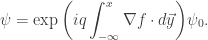
What about the more general case when $\vec{A} \neq \nabla f$ ? The solution can still be written in the form

$\psi = \exp{\left(i q \displaystyle\int_{-\infty}^{x}\vec{A} \cdot d\vec{y}\right)}\psi_{0},$

but now the integral depends on the path taken to reach the point $x$ . This is called a non-integrable phase factor. Let us consider two different paths that arrive at the same point. One can imagine traveling along one, reaching the common end and then continuing around the second path but in the wrong way until one “returns” to infinity. This trip then is around a closed path. We can use Stoke’s theorem for the integral on the exponential for a closed path! Then

$\displaystyle\int_{C_{2}}\vec{A} \cdot d\vec{y} + \displaystyle\int_{-C_{1}}\vec{A} \cdot d\vec{y} = \displaystyle\oint_{\partial \Sigma}\vec{A} \cdot d\vec{y} = \displaystyle\int_{\Sigma}\vec{B}\cdot d\vec{S}.$

Actually it makes sense for this to depend on the magnetic field rather than on the gauge field: this phase factor is physically observable!. For the case of vanishing magnetic field this phase factor becomes unity. But for a more general vector potential, traveling different paths that enclosed some magnetic field flux will get a phase difference between them. This effect is called the Aharonov-Bohm effect.

Finally I would like to comment on different “generalizations” of Maxwell’s theory of electromagnetism. For instance there is Yang-Mills theory. This will require its own two long-winded posts. For now we mention that the field strength $M_{\mu \nu}$ for the Yang-Mills gauge field $Y_{\mu}$ has the form:

$M_{\mu \nu } = \partial_{\mu} Y_{\nu} - \partial_{\nu}Y_{\mu} + [Y_{\mu}, Y_{\nu}].$

Naively one can say that Maxwell theory is the special case of Yang-Mills theory with

$\left[ Y_{\mu} , Y_{\nu} \right] = 0$

This is why Maxwell theory is sometimes known as abelian gauge theory while Yang-Mills is known as non-abelian gauge theory.

I never bothered to write down the Lagrangian for pure electromagnetism. It is easy to understand that it should be gauge invariant and Lorentz invariant. So the best thing we can do is contractions of the field strength with itself. This is another virtue of demanding gauge invariance. For Maxwell theory the Lagrangian is given by

$L = -\displaystyle\frac{1}{4}F^{\mu \nu} F_{\mu \nu}.$

There is a non-linear generalization of Maxwell theory called Born-Infeld theory. The Lagrangian for this theory is given by

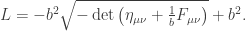
$L = -b^2 \sqrt{-\det{\left(\eta_{\mu \nu} + \frac{1}{b}F_{\mu \nu}\right)}} + b^2 .$

This theory is interesting since it admits a maximun magnitude for the “electric” and “magnetic” fields. In this way charged-particles have a finite self-energy. Maxwell theory is obtained in some small magnitude limit.

And for the end I leave the Kalb-Ramond field. Just as the gauge field $A_{\mu}$ couples to the point-particle in the action

$S_{A} = q \displaystyle\int_{L}d\tau A_{\mu}\frac{dx^{\mu}}{d\tau},$

one can extend (no pun intended!) this notion to extended objects like a string. Then one can work with a gauge field $B_{\mu \nu}$ that couples to the string through a term like

$\displaystyle\int d\tau d\sigma B_{\mu\nu} \frac{\partial x^{\mu}}{\partial \tau}\frac{\partial x^{\nu}}{\partial \sigma}.$

This gauge field is antisymmetric in its two indices and will have a field strenght given by

$H_{\mu\nu\lambda} = \partial_{\mu} B_{\nu\lambda} + \partial_{\nu} B_{\lambda \mu} + \partial_{\lambda} B_{\mu\nu} .$

The field strength is invariant under the change

$B_{\mu \nu} \Rightarrow B_{\mu \nu} + \partial_{\mu}\epsilon_{\nu} - \partial_{\nu} \epsilon_{\mu}.$

The funny thing is that the gauge parameter $\epsilon_{\mu}$ now in turn has an additional gauge invariance: all gauge parameters of the form

$\epsilon_{\mu} + \partial_{\mu} \xi$

will yield the same gauge transformation!

With this I stop. One can also write Maxwell’s equations using differential forms. This can be found elsewhere. I am looking forward to writing a series of post about Yang-Mills theory.

Tags: Electromagnetism

This entry was posted on July 17, 2008 at 4:32 PM and is filed under Gauge theory. You can follow any responses to this entry through the RSS 2.0 feed. You can leave a response, or trackback from your own site.

3 Responses to “Elements of Electromagnetism (II)”

echatav Says:
July 17, 2008 at 10:18 PM | Reply
Thanks for giving the talk today and for writing it up! Let’s try to show that Dirac’s equation is gauge invariant. Dirac’s equation is

$(\gamma^{\mu}(\partial_{\mu}-iqA_{\mu})+im)\psi=0$

First see that

$\partial_{\mu}(exp(iq\lambda)\psi)$
$=exp(iq\lambda)iq(\partial_{\mu}\lambda)\psi+exp(iq\lambda)\partial_{\mu}\psi$
$=exp(iq\lambda)(iq(\partial_{\mu}\lambda)+\partial_{\mu}\psi)$ .

So, if we make the substitutions,

$A_{\mu}\to A_{\mu}+\partial_{\mu}\lambda$ and $\psi\to exp(iq\lambda)\psi$ ,

we get

$(\gamma^{\mu}(\partial_{\mu}-iq(A_{\mu}+\partial_{\mu}\lambda))+im)(exp(iq\lambda)\psi)$
$=exp(iq\lambda)(\gamma^{\mu}(\partial_{\mu}-iqA_{\mu})+im)\psi$
$=exp(iq\lambda)\cdot0=0$ .

So, Dirac’s equation is gauge invariant!
Melvin Eloy Says:
July 18, 2008 at 8:31 AM | Reply
Yay! We should also check the Klein-Gordon case, but it is to early in the morning for that now…
Elements of Electromagnetism (I) « Gauge Theory and All Her Friends Says:
July 24, 2008 at 12:00 AM | Reply
[…] | Tags: Electromagnetism | by Melvin Eloy Electromagnetism is really cute. In this post (and its sequel) my aim is to provide a very broad overview of what physicist mean when they talk about the theory […]